Autonomous Differential Equations

Definition

An ODE is called autonomous if it is independent of it’s independent variable $t$. This is to say an explicit $n$th order autonomous differential equation is of the following form:

\[\frac{d^ny}{dt}=f(y,y',y'',\cdots,y^{(n-1)})\]

ODEs that are dependent on $t$ are called non-autonomous, and a system of autonomous ODEs is called an autonomous system.

Solvability

Despite this simplifying restriction, only first order autonomous equations are solvable in general. Second order autonomous equations are reducible to first order ODEs and can be solved in specific cases. Autonomous equations of higher orders, however, are no more solvable than any other ODE.

First Order Equations

General Solution

Note that any explicit first order autonomous equation:

\[\frac{dy}{dt}=h(y)\]

is separable and so their solution sets are given by their equilibrium points, i.e. the roots of $h(y)$, as well as the solutions to the following integral equation:

\[\int\frac{1}{h(y)}\,dy=t+C\]

Where $C$ is the constant of integration.

Note that the following four sections only consider the real solutions to real valued autonomous ODEs.

Limiting Behavior of Solutions

Recall that a continuous function $f(y)$ can only change signs after passing through a zero. However, due to the Picard–Lindelöf theorem, no non-equilibrium solution $y$ to the ODE $f(y)$ can pass through an equilibrium point. This means their derivative can't pass through zero, and so the solution is always increasing/decreasing:

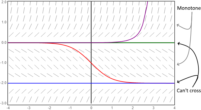
Further, all non-equilibrium solutions approach the nearest equilibrium point or, if none bound it, approach infinity:

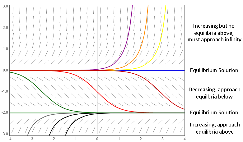
And so, more formally, for any solution $y(t)$ to an autonomous equation $f(y)$ we have the following for an arbitrary point $t_0$ in solution's domain:

• if $f(y(t_0))=0$ then $y(t)$ is a equilibrium solution.
• if $f(y(t_0))>0$ then $y(t)$ is increasing and, as $t\to\infty$, tends to the first equilibrium solution greater than $y(t_0)$ or, if none exist, tends to $\infty$.
• if $f(y(t_0))<0$ then $y(t)$ is decreasing and, as $t\to\infty$, tends to the first equilibrium solution lesser than $y(t_0)$ or, if none exist, tends to $-\infty$.

Note that the limiting behavior is reversed when $t\to-\infty$, we can see this by simply negating the ODE. Also note that this behavior applies only to solutions that satisfy Picard–Lindelöf.

Phase Line

A simple consequence of autonomous ODE's being time independent is that the slopes of the slope field are the same for any time $t$:

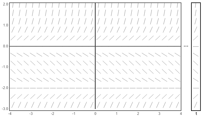
As a result, the graph is redundant in the x-axis and can be encapsulated by a 1-dimensional line parallel to the y-axis. A simplified version of such a plot is called a phase line:

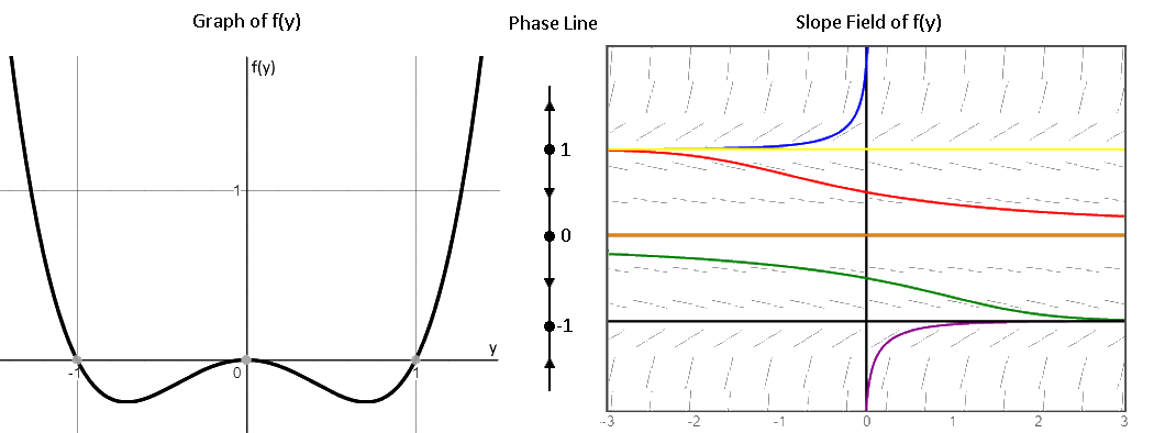
As we can see, the phase line denotes the equilibrium solutions (i.e. the roots of $f(y)$) with a filled in circle while denoting the intervals with increasing/decreasing solutions (i.e. the intervals where $f(y)$ is above/below the $y$-axis) with an up/down arrow.

Phase lines are useful tools in visualizing the properties of particular solutions to autonomous equations. Just by seeing where a solution falls in it, we can tell whether it is increasing, decreasing, or an equilibrium solution. We can also surmise its limiting behavior since it will approach the nearest equilibrium point in the direction it is growing/shrinking. And, if there is no such equilibrium, the solution must grow unbounded.

Classification of Equilibria

As a quick refresher, the equilibria of a first order ODE can be put into three catagories:

• Stable: Solutions sufficiently close to this equilibrium will asymptotically approach it as $t\to\infty$.
• Unstable: Solutions sufficiently close to this equilibrium will diverge from it.
• Semi-stable: Solutions sufficiently close on one side of this equilibrium will asymptotically approach it as $t\to\infty$, but solutions on the other side will diverge from it.

Thanks to the limiting behavior of solutions we discussed earlier, classifying the equilibria of an autonomous equation is as easy as spotting the pattern on its phase line:

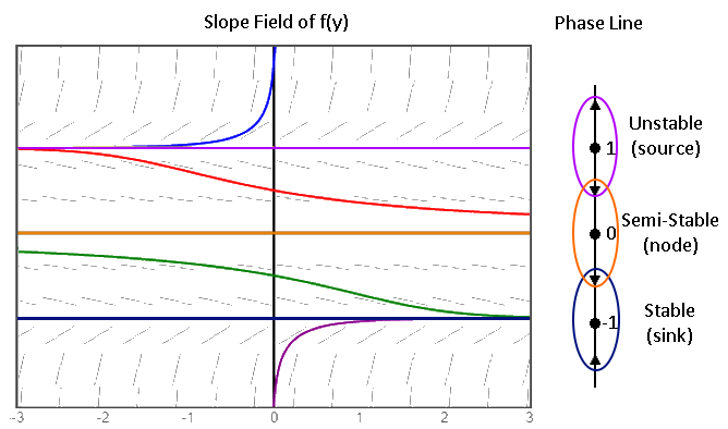
If the surrounding arrows of an equilibrium point point towards it, it is stable (a sink). If they point away from it, it is unstable (a source). And if they point in any other combination, it is semi-stable (a node).

First Derivative Test
For any equilibrium point $y_0$ of an autonomous ODE $f(y)$ we have the following:

• if $f'(y_0)<0$ then $y_0$ is stable (a sink).
• if $f'(y_0)>0$ then $y_0$ is unstable (a source).
• if $f'(y_0)=0$ then the test gives us no information.

Bifurcations

Recall that a bifurcation of a paramaterized family of ODEs $y'=f_\mu(t,y)$ occurs at $\mu=\mu_0$ when the solution set of $f_{\mu_0}(t,y)$ has a different topology than solution sets for values of $\mu$ arbitrarily close to $\mu_0$.

In the case of a family of first order autonomous equations with parameter $\mu$:

$$y'=f_\mu(y)$$

the only kind of bifurcations that can occur are those that change the number/stability of equilibria. And so to visualize these changes, we draw a bifurcation diagram consisting of the following set of points $\mathfrak{B}$ on the $\mu y$ plane:

$$\mathfrak{B}=\{(\mu,y)\in\mathbb R^2\mid f_\mu(y)=0\}$$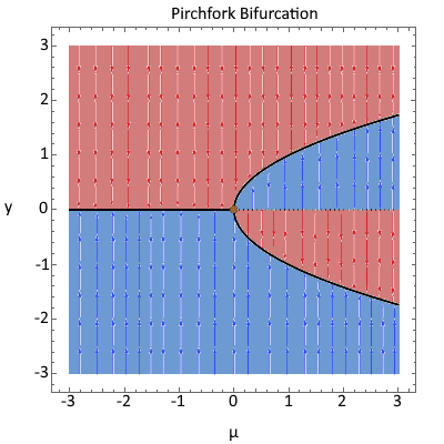

This is a graph of every equilibrium point for every value of $\mu$ and, like a phase line, it makes it easier to spot values and behaviors of interest. In fact, you'll notice that for any particular parameter $\mu_0$, the line $\mu=\mu_0$ is the phase line of the equation $y'=f_{\mu_0}(y)$. You'll also notice that instead of labeling intervals of increasing/decreasing, we shade sectors of increasing/decreasing.

The bifurcation values of the family are simply the values of $\mu$ for which the number/stability of equilibria change. In this case $\mu=0$ is one such value because for $\mu$ after this there are now 2 equilibria rather than 1. This particular type of bifurcation is called a pitchfork bifurcation, and there are other types as well.

Sketching Bifurcation Diagrams

We can graph the equilibria by setting $f_\mu(y)=0$ and solving for $y$ in terms of $\mu$. We must be careful, though, to not lose any points due to things like division by zero.

To shade the sectors appropriately, we simply plug a point from each sector into the differential equation and label it increasing if it is positive and decreasing if it is negative (i.e. we perform the first derivative test). Note that this test will always be conclusive because the only points that won't be either positive or negative, i.e. zero, are the equilibria.

Here is a useful article and paper on bifurcations.

Second Order Equations

As mentioned earlier, higher order autonomous equations are not generally solvable. That said, there are some methods that may work in particular cases. Below we detail one common one for second order autonomous equations.

Order Reduction

A useful method of solving second order autonomous ODEs is expressing them as first order ODEs. We do this by first letting $v=y’$ so that we have:

\[\frac{d^2y}{dt^2}=f(y,v)\]

Now note that, due to the chain rule, we can write:

\[\frac{d^2y}{dt^2}=\frac{dv}{dy}\frac{dy}{dt}=\frac{dv}{dy}v\]

Allowing us to express our original equation as the following first order ODE:

\[\frac{dv}{dy}v=f(y,v)\]

If this ODE is solved, we’ll be left with a solution $v(y)$ which we can then use to solve the following first order autonomous equation:

\[\frac{dy}{dt}=v(y)\]

If we make certain assumptions about the function $f$, like it being separable or dependent only on $y$, we can obtain more explicit solutions for second order autonomous equations.