Breast Cancer Classification

Background

The goal of this project was to implement a neural network from scratch and to train it on a real world dataset pulled from the internet. In this post I’ll attempt to explain the code block by block, as well as a bit of the underlying math, and then finish off by measuring the accuracy of the model.

The model was made with Google’s TensorFlow library, and the entire program is in my NeuralNetwork repository on GitHub as well as at the end of this post.

The Training Data

All the training data comes from the Wisconsin Breast Cancer Data Set, hosted by the University of California’s Machine Learning Repository.

The training data consists of 569 subjects (i.e. breast cancer samples). Each sample is given by a label, benign or malignant, and 30 other values. These values are the mean, worst value, and standard error for each of 10 measurements of the sample:

• Radius (mean of distances from center to points on the perimeter)
• Texture (standard deviation of gray-scale values)
• Perimeter
• Area
• Smoothness (local variation in radius lengths)
• Compactness $(\frac{perimeter^2}{area} - 1)$
• Concavity (severity of concave portions of the contour)
• Concave points (number of concave portions of the contour)
• Symmetry
• Fractal dimension (measure of edge complexity)

It is interesting to note that we don’t really need to know what these values mean and how exactly, if at all, they coorespond to the label of the sample. All we need to know is that they are correlated in some way. Given enough training examples, the neural network will learn how the various variables are related to whether the cell is malignant or benign. This self learning is the essence of machine learning.

All the training examples are stored in a CSV (Comma Separated Value) file called wdbc.data, so our first job is to import the file into our program:

import os #Used for finding file path

#Get dataset file path
path = os.path.dirname(__file__)
file_name = os.path.join(path, 'wdbc.data')
file_object = open(file_name, 'r')

Cleaning the Data

Now that it’s imported, we can start ‘cleaning’ the data. That is, turning this large string of numbers into a list of training examples labeled benign or malignant.

First off we have to split up the dataset, which is currently just one massive string, into a bunch of strings. One for each subject (patient):

#Split dataset into separate points (as strings)
string_points = file_object.read().split('\n')
string_points.pop(-1)

If you take a look at the actual wdbc.data file, you’ll see that some of the subjects are clustered in groups of benign and malignant. If we trained the network with the subjects in this order, it would bias the network’s guesses. To avoid this, we’ll shuffle the subjects:

random.shuffle(string_points) #Randomize (avoid bias)

Next we create a list of feature vectors, each with 30 entries. A feature vector is simply a list of all the data we have about a particular problem, or in this case a particular subject. Its purpose is to be transformed into the desired answer by the neural network. It’s the input.

We will also create a list of $y$ labels ([0,1] for benign and [1,0] for malignant) that correspond with the list of feature vectors. This is the desired output.

We’ll be using the numpy library here, so let’s import it as well:

import numpy as np

num_input_features = 30 #30 data points per subject

#Initialize dataset class arrays
point_array = np.empty((0,num_input_features))
y_labels = np.empty((0,2))

#Trim data points
#Format as np.arrays
#Add to class arrays (Benign or Malignant)
for point in string_points:
    point = point.split(',')
    if 'M' in point: #if malignant
        y_labels = np.append(y_labels, [[0,1]], axis=0)
    else: #if benign (can only be labeled 'B' or 'M')
        y_labels = np.append(y_labels, [[1,0]], axis=0)
    point = point[2:] #trim for only the 10 important features
    temp = np.array(point) #convert to numpy array
    temp = temp.astype(float) #cast as float array
    point_array = np.append(point_array, [temp], axis=0)

All that’s left is to split up the subjects (the list of feature vectors) into training and testing sets. Testing using the same data the network was trained on encourages the network to memorize the data rather than generalize the dataset and make meaningful predictions.

Of the 569 subjects, the first 400 will be used to train the network while the remaining 169 will be used to test the network’s accuracy:

#Split training and testing data
experience_matrix = point_array[0:400]
experience_matrix_y = y_labels[0:400]
test_matrix = point_array[400:]
test_matrix_y = y_labels[400:]

Constructing the Network

A single layer perceptron network seems to do well enough in fitting the test data, so we’ll build one here. The standard model for such a network is given by:

\[\hat{y}=\text{softmax}(Wx+b)\]

• $x$ is the input (a 30 dimensional vector of all the cancer cell’s statistical values).
• $\hat{y}$ is the network’s approximation of $y$, the right answer. (a $2$D vector with the first/second value corresponding to its confidence that the cell is benign/malignant).
• $W$ is a matrix of weights (the matrix is $30\times2$ so that it transforms $30$ dimensional vectors into $2$ dimensional ones).
• $b$ is a vector of ‘bias’ values (a $2$D vector that allows the network more freedom when training, similar to the y-intercept in a linear equation).
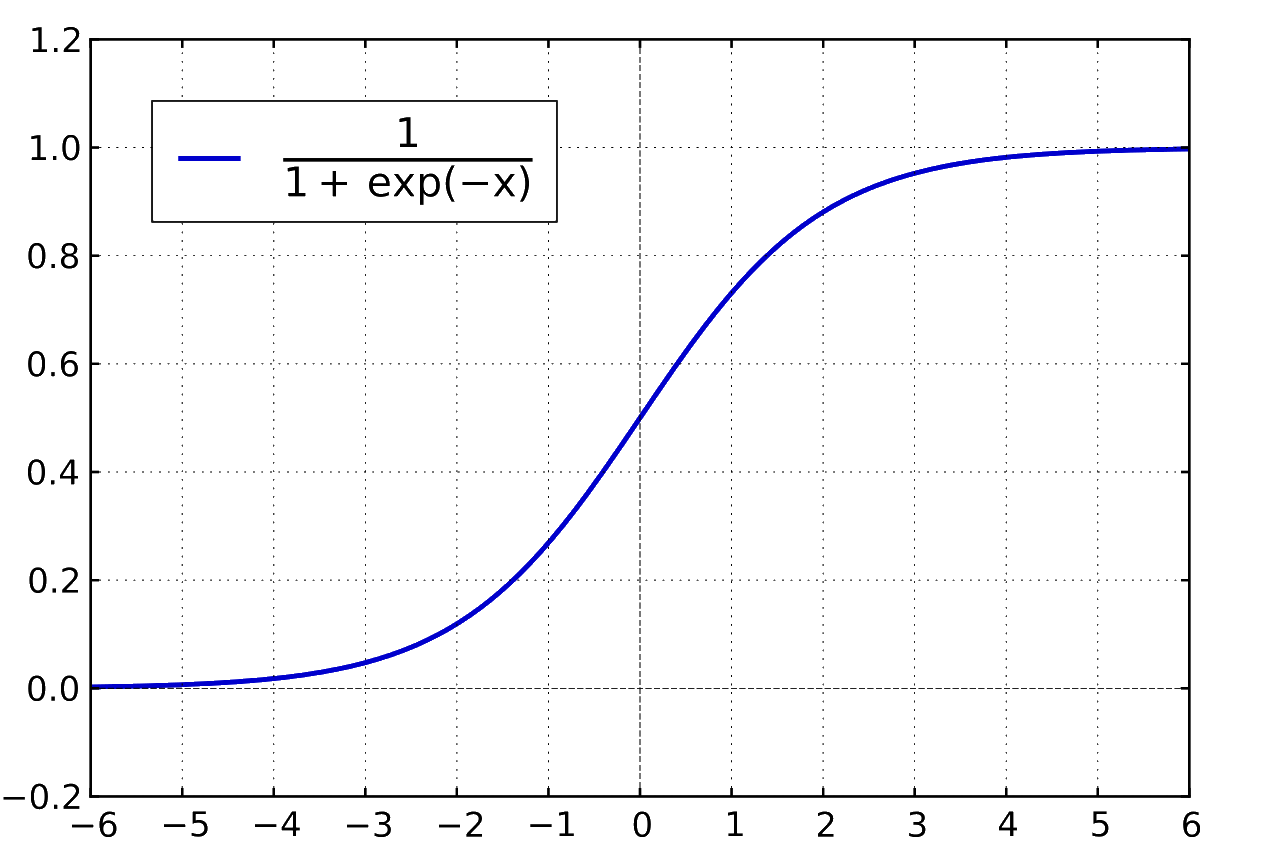
• The $\text{softmax}$ function is the network’s activation function, which introduces a nonlinearity to the network. This is integral for any neural network to learn from the data it’s provided. The function also equalizes the network’s confidence predictions so that they add up to 100%. The mathematical description of softmax is:

Here’s what the model looks like in python with TensorFlow:

import tensorflow as tf

#nx10 Matrix (Input)
  x = tf.placeholder(tf.float32, shape=[None, num_input_features])
#10x1 Matrix (Weights)
  W = tf.Variable(tf.zeros([num_input_features,2]))
#1x2 vector (Bias)
  b = tf.Variable(tf.zeros([2]))
#A scalar (x*W + b)
  y_noSoftmax = tf.matmul(x,W) + b

#Apply softmax (scales y_noSoftmax to be between 0 & 1)
y_hat = tf.nn.softmax(y_noSoftmax, name='y_Hat')

Note that we’ve computed $Wx+b$ first before computing its $\text{softmax}$. Separating these steps will allow us to compute the error function more easily with the TensorFlow library later on.

Training the Network

Now that we’ve assembled the network, we need to train it using the training data, or experience_matrix, and the associated training labels we made earlier.

TensorFlow works by creating what is called a computational graph from which it can calculate and find derivatives of every value in the network, thereby allowing it to optimize (i.e teach) the neural network via backpropagation (Christopher Olah’s blog has a great post on this).

And so, the network won’t start until we create a new graph (session) on which all the training calculations can run:

#Session
sess = tf.InteractiveSession() #Create Session
sess.run(tf.global_variables_initializer()) #Init Variables

Next we create the actual training model. First we create a placeholder for the labels of the training data, $y$.

#nx2 Matrix (One-Hot Vector, Label Data)
y = tf.placeholder(tf.float32, shape=[None, 2],name='y_Labeled')

Then we create a loss function. A loss function is basically a measure of how off the network is in its guesses. This means the smaller the output of this function, the more accurate our network becomes. So, naturally, if we minimize this function we will have effectively trained the network. This is deep learning in a nutshell. Here we use Cross Entropy, as it works nicely with the softmax layer we have at the end.

#Loss Function (cross entropy between y and y_hat)
cross_entropy = tf.reduce_mean(tf.nn.softmax_cross_entropy_with_logits
  (logits = y_noSoftmax, labels = y),name='Loss_Function')

Finally we create the training step. This is where we choose what optimization method to use. In this case we’ll use the tried and true Gradient Descent. I reccommend you look into it yourself, but the gist is that we take partial derivatives of the cost function with respect to every weight variable in the network then slightly adjust them in the direction that would minimize the cost.

This algorithm approaches the local minimum rapidly at first but then slows down once it has gotten close. Here’s a visualization:

And here it is in tensorflow:

#Performs Gradient Descent on loss function
train_step = tf.train.GradientDescentOptimizer(0.5).minimize(
    cross_entropy,name='Train_Step')

Now that we have a training step (a single iteration of gradient descent) we can just run that operation, say, 1000 times for each of the 400 training examples.

#Run train step repeatedly
for i in range(1000):
  #Run training step on the entire batch
    train_step.run(feed_dict={x: experience_matrix, y: experience_matrix_y})

Also note that in the code above, this is where we finally plug our training data (experience_matrix) and labels (experience_matrix_y) into the network. That means that everything we’ve done (in terms of constructing/training the model) can be generalized to many other machine learning problems.

Assessing the Network

To assess how accurate our network is, we simply have to plug in our testing data (test_matrix) and labels (test_matrix_y) into the network and pick the catagory, benign or malignant, that it is most confident in.

First we’ll make a list of Booleans which represent whether the network got the right answer or not:

#Returns whether model made correct prediction (List of booleans)
correct_prediction = tf.equal(tf.argmax(y_hat,1),
    tf.argmax(y,1), name='isCorrect')

Then we average all the results together to arrive at an percent accuracy:

#Average of correct prediction (%Accuracy)
accuracy = tf.reduce_mean(tf.cast
    (correct_prediction,tf.float32),name='Accuracy')

Finally, we just plug in our testing data and labels and print the accuracy (with a bit of pretty formatting) to the console.

#Print Accuracy
print("Accuracy:", '{0:.2%}'.format(accuracy.eval
  (feed_dict={x: test_matrix, y: test_matrix_y})))

When we finally run the code our output should look something like this:

• Accuracy: 90.53%
• Accuracy: 91.12%
• Accuracy: 88.17%

Because we randomized our sample at the start, the accuracy of the network varies slightly each run.

That said the slight increase/decrease in accuracy are just products of how the weights work out with the examples. As such any perceived improvement is probably coincidental and don’t reflect how accurate the network will be in the face of new samples. To get an accurate view of the network’s ability, running it multiple times and taking the average of its accuracy is probably your best bet.

Doing this for our network yields about a 90% accuracy. Not bad. For reference, a monkey (that is, a random process) would classify the cells correctly 50% of the time (there are only two categories). That’s a 40% increase over randomly guessing!

The Full Code

This is all the code put together and is how it appears on my NeuralNetwork repository. All the imports have been moved to the top of the program:

'''
Created on Jun 6, 2017
@author: Ozaner Hansha
'''
import os
import numpy as np
import tensorflow as tf
import random

#Get dataset file path
path = os.path.dirname(__file__)
file_name = os.path.join(path, 'wdbc.data')
file_object = open(file_name, 'r')

#Split dataset into separate points (as strings)
string_points = file_object.read().split('\n')
string_points.pop(-1)
random.shuffle(string_points) #Randomize (avoid bias)

num_input_features = 30

#Initialize dataset class arrays
point_array = np.empty((0,num_input_features))
y_labels = np.empty((0,2))

#Trim data points
#Format as np.arrays
#Add to class arrays (Benign or Malignant)
for point in string_points:
    point = point.split(',')
    if 'M' in point: #if malignant
        y_labels = np.append(y_labels, [[0,1]], axis=0)
    else: #if benign (can only be labeled 'B' or 'M')
        y_labels = np.append(y_labels, [[1,0]], axis=0)
    point = point[2:] #trim for only the 10 important features
    temp = np.array(point) #convert to numpy array
    temp = temp.astype(float) #cast as float array
    point_array = np.append(point_array, [temp], axis=0)

#Split training and testing data
experience_matrix = point_array[0:400]
experience_matrix_y = y_labels[0:400]
test_matrix = point_array[400:]
test_matrix_y = y_labels[400:]

# End of data import/cleanup. Begin construction of neural network
with tf.name_scope('Hidden_Layer'):
  #nx10 Matrix (Input)
    x = tf.placeholder(tf.float32, shape=[None, num_input_features])
  #10x1 Matrix (Weights)
    W = tf.Variable(tf.zeros([num_input_features,2]))
  #1x2 vector (Bias)
    b = tf.Variable(tf.zeros([2]))
  #A scalar (x*W + b)
    y_noSoftmax = tf.matmul(x,W) + b

#Apply softmax (scales y_noSoftmax to be between 0 & 1)
y_hat = tf.nn.softmax(y_noSoftmax, name='y_Hat')

#Session
sess = tf.InteractiveSession() #Create Session
sess.run(tf.global_variables_initializer()) #Init Variables

#Training Model
with tf.name_scope('Training'):
  #nx2 Matrix (One-Hot Vector, Label Data)
    y = tf.placeholder(tf.float32, shape=[None, 2],name='y_Labeled')
  #Loss Function (cross entropy between y and y_hat)
    cross_entropy = tf.reduce_mean(tf.nn.softmax_cross_entropy_with_logits
    (logits = y_noSoftmax, labels = y),name='Loss_Function')
  #Performs Gradient Descent on loss function
    train_step = tf.train.GradientDescentOptimizer(0.5).minimize(
        cross_entropy,name='Train_Step')

#Run train step repeatedly
for i in range(1000):
  #Run training step on that batch
    train_step.run(feed_dict={x: experience_matrix, y: experience_matrix_y})

#Evaluation
with tf.name_scope('Validation'):
  #Returns whether model made correct prediction (List of booleans)
    correct_prediction = tf.equal(tf.argmax(y_hat,1),
        tf.argmax(y,1), name='isCorrect')
  #Average of correct prediction (%Accuracy)
    accuracy = tf.reduce_mean(tf.cast
        (correct_prediction,tf.float32),name='Accuracy')

#Print Accuracy
print("Accuracy:", '{0:.2%}'.format(accuracy.eval
  (feed_dict={x: test_matrix, y: test_matrix_y})))