Expressing Boolean Logic with Matrices

At it’s lowest levels, computation is usually formulated in boolean logic which, in turn, makes use of logical connectives like $\wedge,\vee,$ and $\neg$ along with the binary digits $1$ and $0$, representing true and false respectively.

However, there is an alternative: linear algebra. By representing $0$ and $1$ as vectors and logical operations/gates as matrices, we can define computation in the language of linear algebra. While at first this may seem to be nothing but a novel construction, this reformulation is precisely what opens the door to quantum computing.

0 and 1 states

Instead of $0$ and $1$ or true and false, we instead represent our basic states as the two standard basis vectors in 2-dimensions:

\[\lvert0\rangle = \begin{pmatrix} 1 \\ 0 \\ \end{pmatrix}\quad \lvert1\rangle = \begin{pmatrix} 0 \\ 1 \\ \end{pmatrix}\]

Note the difference between the vector, or state, $\lvert0\rangle$ and the number $0$.¹ As we’ll see below, by multiplying these vectors by matrices we will be able to perform logical operations on them.

Unary Gates

Now that we have a linear algebraic analogue of bits, we will move on to logic gates. Recall that, since a unary gate has only $2$ possible outputs, one for each basis, there are exactly $2^2=4$ unary logic gates. We can represent them as matrices in the following way:

Identity

The identity gate takes an input and returns it as is (i.e $f(x)=x$). To represent it we simply use the $2 \times 2$ identity matrix: $$ I = \begin{pmatrix} 1 & 0 \\ 0 & 1 \end{pmatrix} $$ And indeed, if we apply the gate to both $\lvert 0\rangle$ and $\lvert 1\rangle$ we find: $$\begin{align} I\lvert 0\rangle=\lvert 0\rangle\quad I\lvert 1\rangle=\lvert 1\rangle \end{align}$$

Negation (NOT)

The negation gate takes an input and flips it (i.e $f(x)=\neg x$). We can represent it with the following matrix: $$ \operatorname{NOT} = \begin{pmatrix} 0 & 1 \\ 1 & 0 \end{pmatrix} $$ Applying the gate to both $\lvert 0\rangle$ and $\lvert 1\rangle$ we find: $$\begin{align} \operatorname{NOT}\lvert 0\rangle=\lvert 1\rangle\quad \operatorname{NOT}\lvert 1\rangle=\lvert 0\rangle \end{align}$$

Constant 0

Outputs $0$ regardless of input (i.e $f(x)=0$). We can represent it with the following matrix: $$ C_0 = \begin{pmatrix} 1 & 1 \\ 0 & 0 \end{pmatrix} $$ Applying the gate to both $\lvert 0\rangle$ and $\lvert 1\rangle$ we find: $$\begin{align} C_0\lvert 0\rangle=\lvert 0\rangle\quad C_0\lvert 1\rangle=\lvert 0\rangle \end{align}$$

Constant 1

Outputs $1$ regardless of input (i.e $f(x)=1$). We can represent it with the following matrix: $$ C_1 = \begin{pmatrix} 0 & 0 \\ 1 & 1 \end{pmatrix} $$ Applying the gate to both $\lvert 0\rangle$ and $\lvert 1\rangle$ we find: $$\begin{align} C_1\lvert 0\rangle=\lvert 1\rangle\quad C_1\lvert 1\rangle=\lvert 1\rangle \end{align}$$

Sanity Check

Just as a check, let’s make sure multiplying $\lvert 1\rangle$ by $\operatorname{NOT}$ actually gives $\lvert 0\rangle$ when we write out the matrix multiplication:

\[\operatorname{NOT}\lvert1\rangle=\begin{pmatrix} 0 & 1 \\ 1 & 0 \end{pmatrix} \begin{pmatrix} 0 \\ 1 \\ \end{pmatrix}=\begin{pmatrix} 0+1 \\ 0+0 \\ \end{pmatrix}= \begin{pmatrix} 1 \\ 0 \\ \end{pmatrix}=\lvert0\rangle\]

And indeed it does. If you’d like, you can try verifying if the other matrices give the correct output cooresponding to their logic gate counterpart.

Multiple Bits

Before we can introduce the matrices that correspond to binary operations, we need a way of representing multiple bits as a single vector. This is achieved via the tensor product of the $\lvert 0\rangle$ and $\lvert 1\rangle$ vectors. For example, the two bit state $\lvert 10\rangle$ can be constructed as follows:

\[\begin{pmatrix} 0 \\ 1 \\ \end{pmatrix} \otimes \begin{pmatrix} 1 \\ 0 \\ \end{pmatrix}= \begin{pmatrix} 0\begin{pmatrix} 1 \\ 0 \\ \end{pmatrix} \\ 1\begin{pmatrix} 1 \\ 0 \\ \end{pmatrix} \\ \end{pmatrix}= \begin{pmatrix} 0 \\ 0 \\ 1 \\ 0 \\ \end{pmatrix}\]

Which in bra-ket notation is simply:

\[\lvert 1\rangle\otimes\lvert 0\rangle=\lvert 10\rangle\]

Notice that \({10}_{\text{bin}}=2_{\text{dec}}\) and that the only $1$ in the $\lvert 10\rangle$ vector is at the $2$nd index (indexing starts at $0$). Indeed, it holds true in general that the vector representation of $n$ bits will be a $2^n$ dimensional vector with $0$’s everywhere except for a $1$ at the $i$th index, where $i$ is the value of the bit string.

More explicitly, given an $n$ long bitstring \((x_i)_{i=0}^{n-1}\) such that $(x_0x_1\cdots x_{n-1})_{\text{bin}}=i$, we have the following vector representation:

\[\lvert x_0\rangle\otimes\lvert x_1\rangle\otimes\cdots\otimes\lvert x_{n-1}\rangle=\lvert x_0x_1\cdots x_{n-1}\rangle=\begin{pmatrix} 0 \\ \vdots \\ 0 \\ 1 \\ 0\\ \vdots\\ 0 \end{pmatrix}\begin{matrix} 0\text{th} \\ \vdots \\ (i-1)\text{th} \\ i\text{th} \\ (i+1)\text{th}\\ \vdots\\ (2^n-1)\text{th} \end{matrix}\]

Binary Gates

Now that we can represent bit strings as vectors, it’s possible to construct operations that take in $2$ bits and output $1$ bit. While there are technically $2^{2^2}=16$ possible binary bit operations, we’ll only construct the more useful ones like AND, OR, XOR, etc.

Disjunction (OR)

The $\operatorname{OR}$ gate represents logical disjunction (i.e $f(x,y)=x\vee y$) and is represented by the following matrix: $$ \operatorname{OR} = \begin{pmatrix} 1 & 0 & 0 & 0 \\ 0 & 1 & 1 & 1 \end{pmatrix} $$ Applying the gate to all two bit states we find: $$\begin{align} \operatorname{OR}\lvert 00\rangle&=\lvert 0\rangle & \operatorname{OR}\lvert 01\rangle&=\lvert 1\rangle\\ \operatorname{OR}\lvert 10\rangle&=\lvert 1\rangle & \operatorname{OR}\lvert 11\rangle&=\lvert 1\rangle \end{align}$$

Conjunction (AND)

The $\operatorname{AND}$ gate represents logical conjunction (i.e $f(x,y)=x\wedge y$) and is represented by the following matrix: $$ \operatorname{AND} = \begin{pmatrix} 1 & 1 & 1 & 0 \\ 0 & 0 & 0 & 1 \end{pmatrix} $$ Applying the gate to all two bit states we find: $$\begin{align} \operatorname{AND}\lvert 00\rangle&=\lvert 0\rangle & \operatorname{AND}\lvert 01\rangle&=\lvert 0\rangle\\ \operatorname{AND}\lvert 10\rangle&=\lvert 0\rangle & \operatorname{AND}\lvert 11\rangle&=\lvert 1\rangle \end{align}$$

Exclusive Disjunction (XOR)

The $\operatorname{XOR}$ gate represents exclusive disjunction (i.e $f(x,y)=x\oplus y$) and is represented by the following matrix: $$ \operatorname{XOR} = \begin{pmatrix} 1 & 0 & 0 & 1 \\ 0 & 1 & 1 & 0 \end{pmatrix} $$ Applying the gate to all two bit states we find: $$\begin{align} \operatorname{XOR}\lvert 00\rangle&=\lvert 0\rangle & \operatorname{XOR}\lvert 01\rangle&=\lvert 1\rangle\\ \operatorname{XOR}\lvert 10\rangle&=\lvert 1\rangle & \operatorname{XOR}\lvert 11\rangle&=\lvert 0\rangle \end{align}$$

Logical Equivalence (IFF)

Logical equivalence/biconditional checks if two bits are equal (i.e $f(x,y)=x\iff y$) and is represented by the following matrix: $$ \operatorname{IFF} = \begin{pmatrix} 0 & 1 & 1 & 0 \\ 1 & 0 & 0 & 1 \end{pmatrix} $$ Notice that logical equivalence is the negation of XOR, XNOR (i.e $x\leftrightarrow y=\neg(x\oplus y)$) meaning all the $0$'s and $1$'s in the $\operatorname{XOR}$ matrix are simply swapped to form the equality one. Applying the gate to all two bit states we find: $$\begin{align} \operatorname{IFF}\lvert 00\rangle&=\lvert 1\rangle & \operatorname{IFF}\lvert 01\rangle&=\lvert 0\rangle\\ \operatorname{IFF}\lvert 10\rangle&=\lvert 0\rangle & \operatorname{IFF}\lvert 11\rangle&=\lvert 1\rangle \end{align}$$

Material Implication (IF)

Material implication is a statement of one variable's dependence on another (i.e $f(x,y)=x\implies y$). It's more commonly referred to as an $\operatorname{IF}$ statement in computer science (however this notion of implication is different from the purely logical one above). $$ \operatorname{IF} = \begin{pmatrix} 0 & 0 & 1 & 0 \\ 1 & 1 & 0 & 1 \end{pmatrix} $$ Applying the gate to all two bit states we find: $$\begin{align} \operatorname{IF}\lvert 00\rangle&=\lvert 1\rangle & \operatorname{IF}\lvert 01\rangle&=\lvert 1\rangle\\ \operatorname{IF}\lvert 10\rangle&=\lvert 0\rangle & \operatorname{IF}\lvert 11\rangle&=\lvert 1\rangle \end{align}$$

Sanity Check 2

Just like with the unary gates, let’s use an example to make sure we’re not leading ourselves astray. Consider multiplying the bitstring $\lvert 11\rangle$ by $\operatorname{AND}$. We’d expect it to return $\lvert 1\rangle$, and indeed it does:

\[\operatorname{AND}\lvert11\rangle=\begin{pmatrix} 1 & 1 & 1 & 0 \\ 0 & 0 & 0 & 1 \end{pmatrix} \begin{pmatrix} 0 \\ 0 \\ 0 \\ 1 \end{pmatrix}=\begin{pmatrix} 0+0+0+0 \\ 0+0+0+1 \\ \end{pmatrix}= \begin{pmatrix} 0 \\ 1 \\ \end{pmatrix}=\lvert1\rangle\]

Glorified Truth Tables

Notice that the $i$th column of any one of these matrices is either the $\lvert 0\rangle$ or $\lvert 1\rangle$ vector, depending on what the gate outputs when given the input $i$ in binary form. For example, the $3$rd column of $\operatorname{XOR}$ is $\lvert0\rangle$ which is the output of the XOR when given the input \(11_{\text{bin}}=3_{\text{dec}}\).

Notice that because of this, we can essentially view these matrices as glorified truth tables. And infact, if you look back, this same property held for the unary gates as well. We wrap all this information up below.

Putting it Together

We can now appreciate this new formulation of binary computation for what it is, an isomorphism from Booleans to vectors, logical connectives to matrices, and function composition to matrix multiplication.

In general, the matrix form of a logical operation from $m$ bits to $n$ bits is a $2^m\times 2^n$ matrix whose $i$th column is the output when multiplied by the state $i$ represents. Given an input of the tensor product of $m$ basis vectors, the output is simply their product.

Here’s an example of an operation from 2 bits to 2 to get us accustomed, the half-adder:

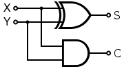
The outputs of the half-adder in terms of logical connectives are $S=X\oplus Y$ and $C=X\wedge Y$, where $S$ is the sum bit and $C$ is the carry bit. Below is an algebraic derivation the matrix representation of the half-adder:

Derivation

To find the matrix that corresponds to sending two bits through a half adder, we must compute the tensor product of $X$ and $Y$ then compute and solve a series of tensor products: $$\begin{align} \text{Let } X&:= \begin{pmatrix} a\\ b \end{pmatrix} \wedge X=\lvert 0\rangle \oplus X=\lvert 1\rangle\\ \text{Let } Y&:= \begin{pmatrix} c\\ d \end{pmatrix} \wedge Y=\lvert 0\rangle \oplus Y=\lvert 1\rangle \end{align}$$ Notice that $X$ must be $\lvert 0\rangle$ xor $\lvert 1\rangle$, and the same for $Y$. This condition is what allows us to solve for the gate. But before we do that let us find the tensor product of $X$ and $Y$ so that we may think of them as a 2 bit input: $$X\otimes Y= \begin{pmatrix} a\\ b \end{pmatrix}\oplus \begin{pmatrix} c\\ d \end{pmatrix}= \begin{pmatrix} a\begin{pmatrix} c \\ d \\ \end{pmatrix} \\ b\begin{pmatrix} c \\ d \\ \end{pmatrix} \\ \end{pmatrix}= \begin{pmatrix} ac \\ ad \\ bc \\ bd \\ \end{pmatrix}$$ The output bits $S$ and $C$ can now be represented as the following equations: $$\begin{align} S&=\operatorname{XOR}(X\otimes Y)= \begin{pmatrix} 1 & 0 & 0 & 1 \\ 0 & 1 & 1 & 0 \end{pmatrix} \begin{pmatrix} ac \\ ad \\ bc \\ bd \end{pmatrix}= \begin{pmatrix} ac+bd \\ ad+bc \end{pmatrix}\\ C&=\operatorname{AND}(X\otimes Y)= \begin{pmatrix} 1 & 1 & 1 & 0 \\ 0 & 0 & 0 & 1 \end{pmatrix} \begin{pmatrix} ac \\ ad \\ bc \\ bd \\ \end{pmatrix}= \begin{pmatrix} ac+ad+bc \\ bd \end{pmatrix}\\ \end{align}$$ Their tensor product, i.e the output of the half-adder given an input of $X\otimes Y$, is the following: $$\begin{align} S\otimes C&= \begin{pmatrix} ac+bd \\ ad+bc \end{pmatrix} \begin{pmatrix} ac+ad+bc \\ bd \end{pmatrix}\\ &=\begin{pmatrix} (ac)^2+a^2cd+abc^2+abcd+abd^2+b^2cd \\ abcd+bd^2\\ a^2cd+(ad)^2+abcd+abcd+(bc)^2\\ abd^2+b^2cd \end{pmatrix} \end{align}$$ While this result may seem unwieldy, recall the stipulation on the vectors $X$ and $Y$ we made when we defined them: they must be each equal to either $\lvert 0\rangle$ or $\lvert 1\rangle$. We can phrase this in terms of their components: $$\begin{align} (a=1\wedge b=0)&\vee(a=0\wedge b=1)\\ (c=1\wedge d=0)&\vee(c=0\wedge d=1) \end{align}$$ Because of this, we can simplify many of the expressions above (example $ab=0$ b.c. either $a$ or $b$ is $0$) to form a more simpler vector: $$\begin{pmatrix} (ac)^2+a^2cd+abc^2+abcd+abd^2+b^2cd \\ abcd+bd^2\\ a^2cd+(ad)^2+abcd+abcd+(bc)^2\\ abd^2+b^2cd \end{pmatrix}=\begin{pmatrix} ac\\ bd\\ bc+ad\\ 0 \end{pmatrix}$$ For those familiar with logic, we can also think of this finding non-contingent statements and simplifying them.

Now we can consider the following equation: $$\operatorname{Half-Adder}(X\otimes Y)=(S\otimes C)$$ We can solve for the $\operatorname{Half-Adder}$ matrix by explicitly writing out the above equation: $$ \begin{pmatrix} ? &? &? &?\\ ? &? &? &?\\ ? &? &? &?\\ ? &? &? &? \end{pmatrix} \begin{pmatrix} ac \\ ad \\ bc \\ bd \\ \end{pmatrix} =\begin{pmatrix} ac\\ bd\\ bc+ad\\ 0 \end{pmatrix}$$ From the rules of matrix multiplication, it should be clear that the sole matrix that solves this equation is: $$\begin{pmatrix} 1 & 0 & 0 & 0 \\ 0 & 0 & 0 & 1 \\ 0 & 1 & 1 & 0 \\ 0 & 0 & 0 & 0 \end{pmatrix}$$

Recall though that the above derivation isn’t necessary since we can simply construct a truth table for the circuit and construct the matrix from it, setting the $i$th column as the output of the half-adder given the input $i$. Doing this we arrive at the following:

\[\text{Half-Adder}= \begin{pmatrix} 1 & 0 & 0 & 0 \\ 0 & 0 & 0 & 1 \\ 0 & 1 & 1 & 0 \\ 0 & 0 & 0 & 0 \end{pmatrix}\]

CNOT and the Echoes of Quantum Computing

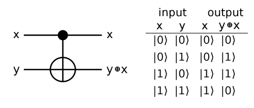
As a final example, and lead-in to quantum computing, I’ll describe another 2 bit to 2 bit logic gate²: the controlled NOT or CNOT gate.

Its function is pretty simple: the gate acts as a NOT gate on the second bit, but only if the first bit is $1$. If this first bit, dubbed the control bit, is $0$ then the second bit, dubbed the target bit, won’t be affected at all. The first unchanged bit and the second possibly negated bit are then outputted. The circuit notation and truth table looks like this:

Using the truth table to form a matrix we have:

\[\text{CNOT} = \begin{pmatrix} 1 & 0 & 0 & 0 \\ 0 & 1 & 0 & 0 \\ 0 & 0 & 0 & 1 \\ 0 & 0 & 1 & 0 \end{pmatrix}\]

While this gate may not seem particularly interesting, and indeed it isn’t as far as classical computing is concerned, its real power shows when the control bit, or rather qubit³, is in a quantum superposition of both $\lvert 0\rangle$ and $\lvert 1\rangle$, ala quantum computing. If that were the case, then what would the target bit be?

In quantum mechanics we’d call such system of qubits entangled since, while we don’t know what each qubit’s state will be before we look, after looking at just one of the qubits we’d instantly know what the other is. For example, if the target was unchanged then the control must be $\lvert 0\rangle$.

But we’ll unpack all this in a later post…

1. Referring to states using these brackets, known as bra-ket notation, is standard in quantum mechanics and thus in quantum computing as well. ↩

2. While we could construct logic gates of arbitrary size, the logical operations we study in both classical and quantum computing usually only have inputs/outputs of 2 bits max. This makes sense given that more complicated gates and operations can be built from these simpler ones. ↩

3. As in quantum bits. While it doesn’t make sense to have a bit in a superposition of both $\lvert 0\rangle$ and $\lvert 1\rangle$, this is commonplace for a qubit. ↩